Intro to Making Publication Style Tables Using Esttab
Estimate Tables
Being able to present regression results in a clean, concise way is a skill almost as important as running the regressions themselves. You will never see a screenshot of STATA in a journal or when an author presents their work. Yet, there isn’t a class that will formally teach you how to create publication quality tables. This guide is meant to be a very brief introduction to producing exportable regression tables using STATA.
For demonstration purposes, I will be estimating a Differences-in-Differences model that aims to measure the effects of the Familias en Accion condition cash transfer program on neo-natal health in Colombia. The Health Economics literature suggests that low birth weight is a strong predictor of poor human capital development later on in life. As such, policies that improve in-utero health can be very useful (and often cost effective) development programs. You can download the data here to play with and follow along.
Nota Bene: This will in no way, shape or form affect your grade, but it is best practice, and will be extremely useful if you go on to do graduate economics. If that is your plan, learning how to make estimate tables is definitely worth the time investment. There are similar workflows for R, but I will stick to STATA since it is most common.
eststo/esttab/estout
The most common, and in my experience most effective, workflow for creating publication quality tables is using the eststo, esttab, and estout commands. There is a similar workflow that uses the outreg command, but I find it a little more cumbersome and a little less flexible.
The basic idea of the eststo/esttab/estout workflow is that you “store” estimates from regression results using the eststo command, and then combine the estimates you have stored into a single table, where each column has the results of one regression model, using the esttab command. This table can easily then be exported from STATA to Word, Excel, or LateX.
I will cover the very basics to get you going, but the documentation is available here. There are tons of things you can do with these commands, and the documentation is fantastic.
Installation
To get started, install the necessary packages by running the command:
ssc install estout
And you’re good to go!
Storing Estimates
To store estimates, we use the eststo command. Let’s use a differences-in-differences model to with year FE as an example. Note that I am using the aweight command to weight the municipality level observations by the the weight variable, which is proportional to the number of births in a municipality. Further, I am clustering the standard errors at the municipality level using vce(cluster codmpio).
There are two ways to store the estimates using eststo:
reghdfe lbw did treat [aweight = weight], absorb(year) vce(cluster codmpio)
eststo did_yfe
or (my prefered syntax):
eststo did_yfe: reghdfe lbw did treat [aweight = weight], absorb(year) vce(cluster codmpio)
Once you have run this, the results will be stored under the name did_yfe that you can call upon when you create the estimate table. There is more you can do with the command, but this is all you will be doing 90% of the time. Note that naming is technically optional, and you can choose to leave it out - don’t do that, future you will hate you.
Creating an Estimate Table
Say you have run a number of different models and haves stored them. You can now create an estimate table! To do this, we use the esttab command. For this example, I have estimated a series of models where I vary the fixed effects and controls used. They are saved under the names did, did_yfe, did_mfe, did_myfe, and did_myfe_control. To create an estimate table, you can run the command:
esttab did did_yfe did_mfe did_myfe did_myfe_control
This will produce a rather crude table, with t-stats instead of standard errors and the “wrong” significance stars! We can easily fix all of that by adding some options to the command
sewill add standard errors in parenthesislabelwill use variable labels instead of names. Please use labels. No one wants to be guessing what lnhct_1_pc_4rtk means….keepwill let you specify what coefficients you want to report. In this case, we do not care about the constant, and will omit it.star(* 0.10 ** 0.05 *** 0.01)will produce the usual star system that we use by (outdated, wrong) convention.
Adding these options will make your command look like this:
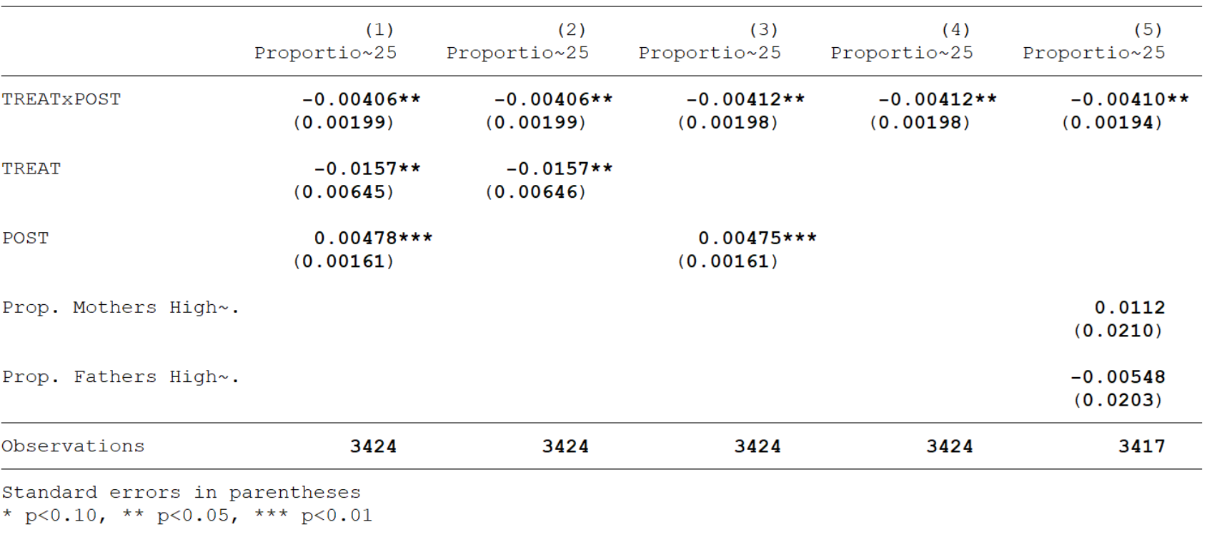
esttab did did_yfe did_mfe did_myfe did_myfe_control, label se star(* 0.10 ** 0.05 *** 0.01) keep(did treat post mat_hs_v pat_hs_v)
We now have a table that actually looks like something you might see in a paper!
estadd - a very useful addition!
Say there is some extra information about your model that you want to share in your table. In that case, estadd can be incredibly useful. For example, you may want to make it clear to your reader what fixed effects you are using in a specific regression. To do this, you can add a local macro to your stored estimate. This will look something like this:
eststo did_mfe: reghdfe lbw did post [aweight = weight], absorb(codmpio) vce(cluster codmpio)
quietly estadd local fixedm "Yes", replace
quietly estadd local fixedy "No", replace
What we have done here is created a local macro named fixedm that takes value “Yes” for this regression because we are using municipality fixed effects, and similarly fixedy for year fixed effects which takes value “No”. We will include these macros in the table as rows later using esttab. Note that I include replace as an option - this is to tell STATA to overwrite anything that is already written in that spot.
In addition to indicating fixed effects, we can use estadd to add calculated statistics. This will often be the mean of the dependent variable, as we will do for these results. Reporting the mean of the dependent variable in a table helps the reader understand the magnitude of a calculated effect. To do this, the command estadd ysumm tells stata to store the summary statistics of the outcome variable, to be called upon later.
eststo did_mfe: reghdfe lbw did post [aweight = weight], absorb(codmpio) vce(cluster codmpio)
quietly estadd local fixedm "Yes", replace
quietly estadd local fixedy "No", replace
estadd ysumm, replace
We can also use estadd to add statistics that are calculated from estimate results (usually some transformation of $\beta$ coefficients).
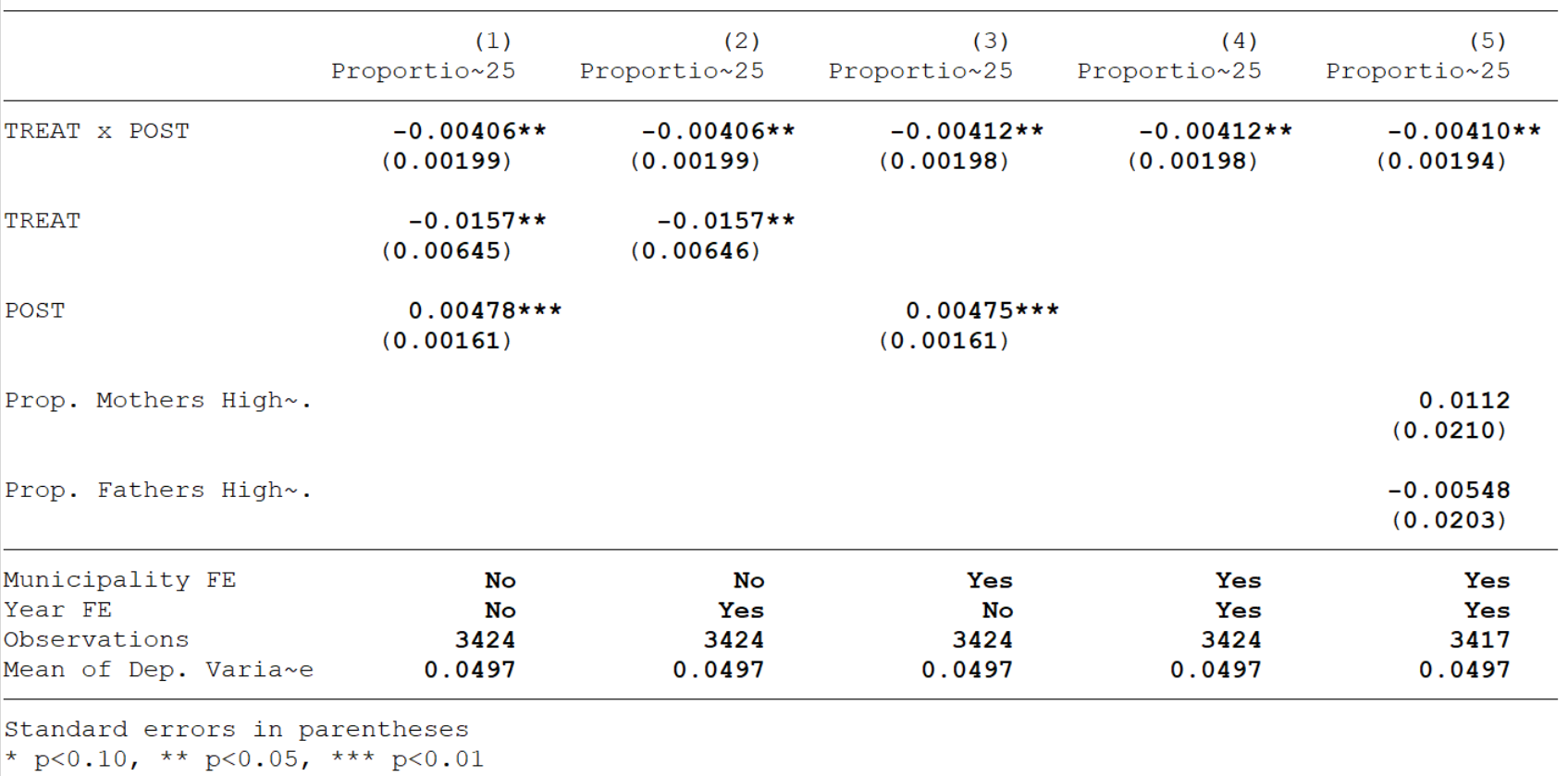
Once we have run these, we can create a table that includes this additional information. To do this, we use the scalars option. We need to list the scalar/locals that we want, and give the rows names using the label suboption. There are some scalars that are automatically stored. For example, N will give you number of observations. ymean will call upon the mean of the dependent variable, that we had stored using ysumm. The command will look like this:
esttab did did_yfe did_mfe did_myfe did_myfe_control using "sample_reg_table.rtf", replace label se star(* 0.10 ** 0.05 *** 0.01)s(fixedm fixedy N ymean,label("Municipality FE" "Year FE" "Observations" "Mean of Dep. Variable")) keep(did treat post mat_hs_v pat_hs_v);
Bonus Tip!!! This is an unreadably long line… what we can do is change the delimiter to a semicolon. The #delimit ; command tells STATA that from that point forward, a line is not over until it has seen a semicolon. When we are done with our absurdly long command, we can make the delimiter a carriage return (what old people call enter because of typewriters) again using the #delimit cr command. Much better:
#delimit ;
esttab did did_yfe did_mfe did_myfe did_myfe_control using "sample_reg_table.rtf",
	replace label se star(* 0.10 ** 0.05 *** 0.01)
	s(fixedm fixedy N ymean,
	label("Municipality FE" "Year FE" "Observations" "Mean of Dep. Variable"))
	keep(did treat post mat_hs_v pat_hs_v);
#delimit cr
This produces the exact table that we want to be showing people. Looks good, huh?
Exporting to Word
The real beauty of esttab is that it makes it easy to export the table to your favourite typesetter. If you want to use the table in Word, simply add using filename.rtf to your command. If you specify just a filename, the rtf document will be placed in your current directory. Alternatively, you can use a full file path to specify where you want the table saved. The code should look like this:
#delimit ;
esttab did did_yfe did_mfe did_myfe did_myfe_control using "sample_reg_table.rtf",
	replace label se star(* 0.10 ** 0.05 *** 0.01)
	s(fixedm fixedy N ymean,
	label("Municipality FE" "Year FE" "Observations" "Mean of Dep. Variable"))
	keep(did treat post mat_hs_v pat_hs_v);
#delimit cr
Note that I include the replace option. This is so that STATA will overwrite any existing file of that name (otherwise it will yell at you if you run your code more than once). You can also export to Excel, I find that .csv works better than .xls, but to each their own. The table will open up in Word like this:
Exporting to LaTeX
esttab can also make LaTeX tables for you! Run the following code and it will create a .tex file that contains the table. You can either copy-paste this into your source code - or better yet, reference it in the code using the \include() command. If you do that, every time you update your results and STATA replaces the output table, the results in your paper update automatically. In my opinion, this is the ideal workflow.
#delimit ;
esttab did did_yfe did_mfe did_myfe did_myfe_control using "sample_reg_table.tex",
   replace label se star(* 0.10 ** 0.05 *** 0.01)
   s(fixedm fixedy N ymean,
   label("Municipality FE" "Year FE" "Observations" "Mean of Dep. Variable"))
   keep(did treat post mat_hs_v pat_hs_v);
#delimit cr
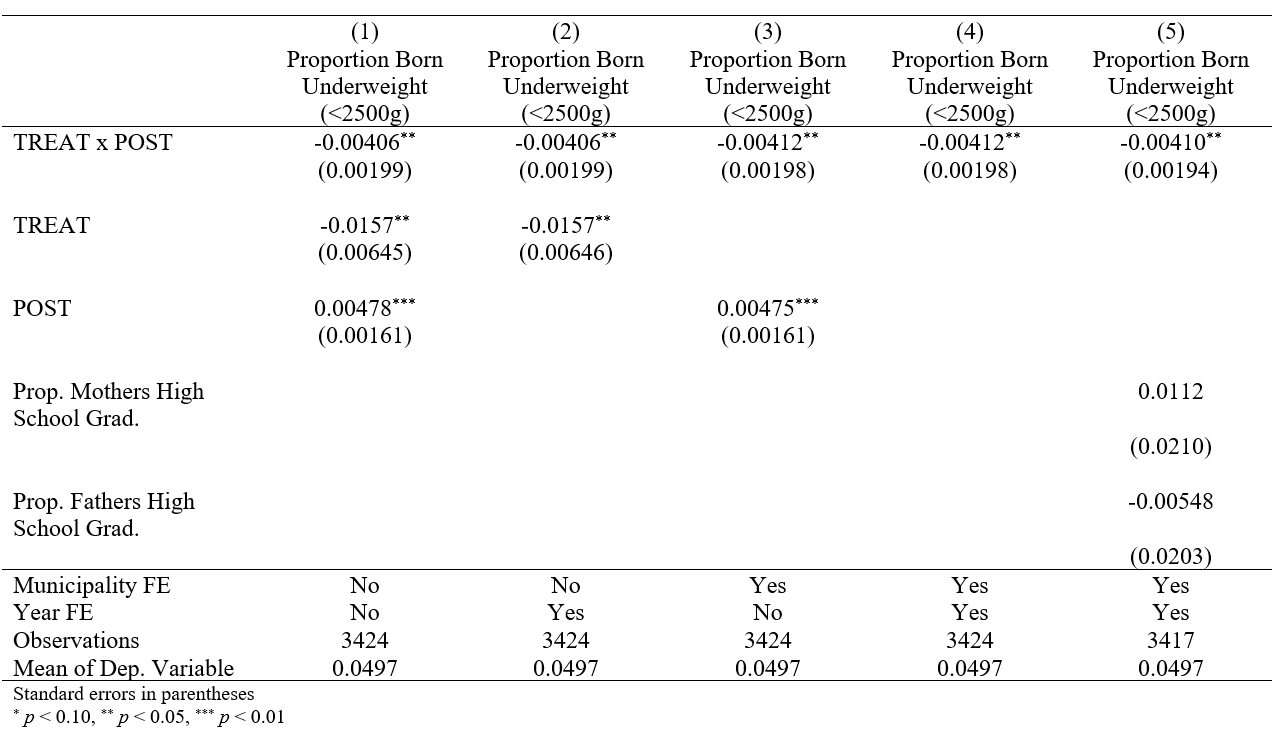
The output file that this command produces will look like this - much easier than manually creating a table in LaTeX. You can also create booktabs tables (simply add the booktabs option in the esttab command and make sure you are loading the correct packages in your .tex file). Booktabs tables look much nicer than the .tex default.
{
\def\sym#1{\ifmmode^{#1}\else\(^{#1}\)\fi}
\begin{tabular}{l*{5}{c}}
\hline\hline
                    &\multicolumn{1}{c}{(1)}&\multicolumn{1}{c}{(2)}&\multicolumn{1}{c}{(3)}&\multicolumn{1}{c}{(4)}&\multicolumn{1}{c}{(5)}\\
                    &\multicolumn{1}{c}{Proportion Born Underweight (<2500g)}&\multicolumn{1}{c}{Proportion Born Underweight (<2500g)}&\multicolumn{1}{c}{Proportion Born Underweight (<2500g)}&\multicolumn{1}{c}{Proportion Born Underweight (<2500g)}&\multicolumn{1}{c}{Proportion Born Underweight (<2500g)}\\
\hline
TREAT x POST        &    -0.00406\sym{**} &    -0.00406\sym{**} &    -0.00412\sym{**} &    -0.00412\sym{**} &    -0.00410\sym{**} \\
                    &   (0.00199)         &   (0.00199)         &   (0.00198)         &   (0.00198)         &   (0.00194)         \\
[1em]
TREAT               &     -0.0157\sym{**} &     -0.0157\sym{**} &                     &                     &                     \\
                    &   (0.00645)         &   (0.00646)         &                     &                     &                     \\
[1em]
POST                &     0.00478\sym{***}&                     &     0.00475\sym{***}&                     &                     \\
                    &   (0.00161)         &                     &   (0.00161)         &                     &                     \\
[1em]
Prop. Mothers High School Grad.&                     &                     &                     &                     &      0.0112         \\
                    &                     &                     &                     &                     &    (0.0210)         \\
[1em]
Prop. Fathers High School Grad.&                     &                     &                     &                     &    -0.00548         \\
                    &                     &                     &                     &                     &    (0.0203)         \\
\hline
Municipality FE     &          No         &          No         &         Yes         &         Yes         &         Yes         \\
Year FE             &          No         &         Yes         &          No         &         Yes         &         Yes         \\
Observations        &        3424         &        3424         &        3424         &        3424         &        3417         \\
Mean of Dep. Variable&      0.0497         &      0.0497         &      0.0497         &      0.0497         &      0.0497         \\
\hline\hline
\multicolumn{6}{l}{\footnotesize Standard errors in parentheses}\\
\multicolumn{6}{l}{\footnotesize \sym{*} \(p<0.10\), \sym{**} \(p<0.05\), \sym{***} \(p<0.01\)}\\
\end{tabular}
}
Sample Code
****************************************************
*         USING ESTTAB FOR REGRESSION TABLES       *
*                 AUTHOR: DARIO TOMAN              *
*               	Sample Code                *
*                                                  *
****************************************************

* This code is meant as an aid - there are n+1 ways to do things in STATA

clear all
set more off

*Begin by loading data
use "Sample_data_FeA.dta"

*Generate variables that are needed for Differences-in-Differences Analysis
gen treat = (FeA_year_reg==2001)
gen post = (year > 2000)
gen did = treat*post

label variable did "TREAT x POST"
label variable treat "TREAT"
label variable post "POST"

****************************************************
*                    Regressions       	           *
****************************************************
eststo did: reghdfe lbw did treat post[aweight = weight], noabsorb vce(cluster codmpio)
estadd local fixedm "No", replace
estadd local fixedy "No", replace
estadd ysumm, replace

eststo did_yfe: reghdfe lbw did treat [aweight = weight], absorb(year) vce(cluster codmpio)
quietly estadd local fixedm "No", replace
quietly estadd local fixedy "Yes", replace
estadd ysumm, replace

eststo did_mfe: reghdfe lbw did post [aweight = weight], absorb(codmpio) vce(cluster codmpio)
quietly estadd local fixedm "Yes", replace
quietly estadd local fixedy "No", replace
estadd ysumm, replace

eststo did_myfe: reghdfe lbw did [aweight = weight], absorb(codmpio year) vce(cluster codmpio)
quietly estadd local fixedm "Yes", replace
quietly estadd local fixedy "Yes", replace
estadd ysumm, replace

eststo did_myfe_control: reghdfe lbw did mat_hs_v pat_hs_v [aweight = weight], absorb(codmpio year) vce(cluster codmpio)
quietly estadd local fixedm "Yes", replace
quietly estadd local fixedy "Yes", replace
estadd ysumm, replace


esttab, label


****************************************************
*                       TABLE         	           *
****************************************************

*I can now use the esttab function to generate one table that will have all of
*the results.

#delimit ;
esttab did did_yfe did_mfe did_myfe did_myfe_control, label se star(* 0.10 ** 0.05 *** 0.01)
	s(fixedm fixedy N ymean,
	label("Municipality FE" "Year FE" "Observations" "Mean of Dep. Variable"))
	keep(did treat post mat_hs_v pat_hs_v);
#delimit cr


* I can export this table to an .rtf file that can be pasted into word

#delimit ;
esttab did did_yfe did_mfe did_myfe did_myfe_control using "sample_reg_table.rtf",
	replace label se star(* 0.10 ** 0.05 *** 0.01)
	s(fixedm fixedy N ymean,
	label("Municipality FE" "Year FE" "Observations" "Mean of Dep. Variable"))
	keep(did treat post mat_hs_v pat_hs_v);
#delimit cr


* Or LateX if I'm feeling ~*~fancy ~*~

#delimit ;
esttab did did_yfe did_mfe did_myfe did_myfe_control using "sample_reg_table.tex",
	replace label se star(* 0.10 ** 0.05 *** 0.01)
	s(fixedm fixedy N ymean,
	label("Municipality FE" "Year FE" "Observations" "Mean of Dep. Variable"))
	keep(did treat post mat_hs_v pat_hs_v);
#delimit cr